Perturbation Theory
Perturbation theory is a fundamental mathematical method in quantum mechanics used to approximate the behavior of complex systems under small disturbances, called perturbations. It is divided into time-independent and time-dependent forms, depending on whether the disturbance varies with time. In time-independent perturbation theory, static disturbances modify the Hamiltonian, allowing physicists to compute corrected energy levels and wavefunctions through first- and second-order corrections. In contrast, time-dependent perturbation theory deals with time-varying fields and interactions—such as photon absorption, stimulated emission, and atomic transitions—and calculates transition probabilities using Fermi’s Golden Rule. This theory underpins major concepts in atomic physics, spectroscopy, and quantum field theory, providing insight into fine-structure corrections, Stark effects, and particle scattering phenomena.
Perturbation Theory
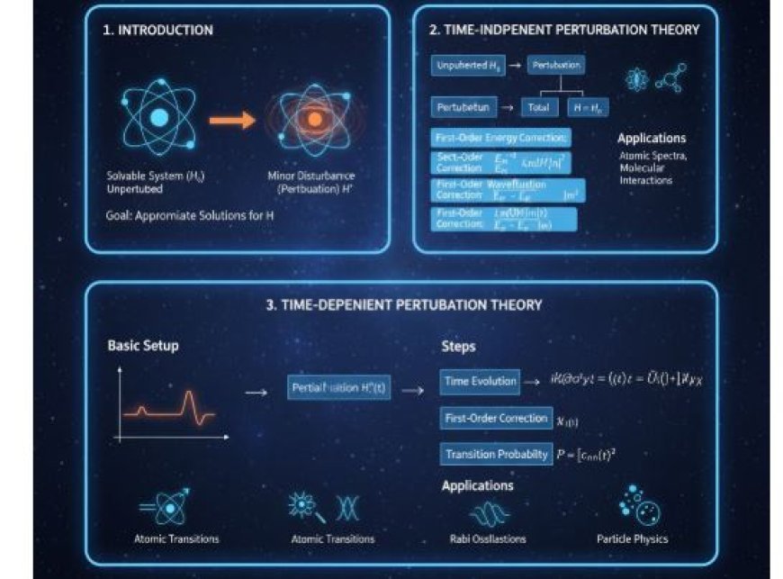
1. Introduction
Perturbation theory is a mathematical approach used in quantum mechanics to estimate the behavior of a system when subjected to a minor disturbance, known as a perturbation. It can be time-dependent or time-independent.
The system is often believed to be solvable exactly in the absence of the perturbation, and the perturbation is viewed as a minor adjustment to the exact solution. Perturbation theory is classified into two types: time-independent and time-dependent. These methods are utilized based on whether the disturbance varies over time or not.
2. Time-Independent Perturbation Theory
This is the most prevalent type of perturbation theory, and it applies when the system is subjected to a constant disturbance. Time-independent perturbation theory is useful for systems in which a modest static disturbance changes the Hamiltonian (the total energy operator).
Basic Setup
- The system's unperturbed Hamiltonian (H₀): Normally solvable and has known eigenvalues and eigenstates.
- Perturbation Hamiltonian (H′): A tiny disturbance added to the system, causing it to deviate somewhat from the initial, solvable system.
- The system's total Hamiltonian:
![]()
where H₀ represents the unperturbed Hamiltonian and H′ represents the perturbation.
Goal
The goal is to identify the corrected eigenvalues and eigenstates of the total Hamiltonian H. Since H₀ is solvable, we start by solving it.
Steps in Time-Independent Perturbation Theory
- Eigenvalues and Eigenstates for H₀:
Solve the unperturbed Hamiltonian H₀ to obtain the energy eigenvalues
![]()
and eigenstates

- First-Order Energy Correction:
The first-order correction for energy Eₙ(1) is defined as the expectation value of the perturbation in the unperturbed state:

- Second-Order Energy Correction:
A second-order adjustment to the energy Eₙ(2) is calculated using the formula:

- First-Order Wavefunction Correction:
To correct the wavefunction ∣n(1)⟩|n^{(1)}\rangle∣n(1)⟩, use the formula:

- Higher-Order Corrections:
Similar recursive relations can be used to compute higher-order adjustments.
Applications
- Atomic spectra and energy levels, including fine structural splitting owing to relativistic effects.
- Understanding molecular interactions and chemical processes.
3. Time-Dependent Perturbation Theory
When a perturbation changes over time, such as an external time-varying electric field or a time-dependent interaction, time-dependent perturbation theory is applied.
Basic Setup
The whole Hamiltonian is now time-dependent:
![]()
where H′(t) represents a time-dependent perturbation.
Goal
Time-dependent perturbation theory seeks to determine how the system changes over time in response to a time-varying disturbance.
Steps in Time-Dependent Perturbation Theory
- Unperturbed State:
Assume an initial unperturbed state
![]()
which evolves according to the unperturbed Hamiltonian H₀.
- Time Evolution Operator:
The Schrödinger equation governs the state's development throughout time:

where ψ(t) is the state vector at time t.
- First-Order Approximation:
Assume the perturbation is small and write the wavefunction as a series expansion in powers of perturbation:
![]()
where ψ₀(t) is the solution to the unperturbed system, and ψ₁(t), ψ₂(t), etc., are corrections due to the perturbation.
- First-Order Wavefunction Correction:
At first order, the wavefunction correction ψ₁(t) is given by:

- Transition Probability:
The squared modulus of the transition amplitude determines the probability of the system being in state |m⟩ at time t from state |n⟩:
![]()
- Second-Order Approximation:
This approach incorporates perturbation adjustments into a higher-order integral, resulting in more accurate predictions of the system's temporal evolution.
Applications
- Atomic transitions: Time-dependent perturbation theory models photon absorption or emission when an atom interacts with an electromagnetic field, such as light absorption or stimulated emission.
- Rabi oscillations: May be described using time-dependent perturbation theory in quantum systems with oscillating fields, such as in quantum optics.
- Particle physics: Scattering amplitudes may be calculated using time-dependent perturbation theory, which considers how particle interactions evolve over time.
Explore Subject Categories
• StudySpot360 Home: https://studyspot360.com/
• Geology Study Materials: https://studyspot360.com/geology
• Physics Notes and Learning Resources: https://studyspot360.com/physics
• English Grammar and Study Materials: https://studyspot360.com/english
About StudySpot360
StudySpot360 is a trusted educational platform providing high-quality study materials, detailed notes, MCQs, quizzes, question papers, and academic resources across multiple subjects. Our mission is to make reliable educational content accessible to students, educators, researchers, and lifelong learners while supporting academic excellence, examination preparation, and continuous learning.
Explore more educational articles, tutorials, practice questions, quizzes, and subject-wise learning resources to strengthen your knowledge and continue your learning journey with StudySpot360.