Orthonormal Normalisation Technique

The Orthonormal Normalisation Technique is a method used in physics to ensure that certain functions or vectors have specific properties. The term "orthonormal" means that the functions or vectors are both:

• Orthogonal (they do not affect each other)
• Normalised (they have a length of one)
• Normalisation is an important concept in many areas of physics, especially in quantum mechanics and statistical physics.
• One notable normalisation method is the orthonormal technique.

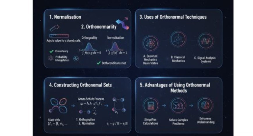
1. Normalisation

Normalisation is a mathematical method used to adjust values recorded on different scales to a notionally shared scale. In physics, it is often used to ensure that quantities like wave functions or probability distributions meet specific physical requirements.

Significance

• Consistency: Ensures that results are uniform and comparable.
• Probability Interpretation: In quantum physics, normalisation helps us understand wave functions as probabilities.

2. Orthonormality

The term "orthonormal" combines two key ideas:

• Orthogonality: Two functions or vectors are orthogonal if their inner product equals zero, meaning they are perpendicular in vector space.
• Normalisation: A function or vector is normal if its length (norm) equals one.

Mathematical Representation

For two functions, f(x) and g(x):

• Orthogonality:
  ∫ f(x) g(x) dx = 0
• Normalisation:
  ∫ |f(x)|² dx = 1

If both conditions are met, then f(x) and g(x) are orthonormal.

3. Uses of Orthonormal Techniques

A. Quantum Mechanics

• Wave Functions:
  • In a Hilbert space, a group of wave functions is orthonormal if the following conditions hold:
    1. The inner product of any two different wave functions is zero.
    2. The inner product of a wave function with itself is one.
• Basis States:
  • Special functions that help describe other states, making calculations and predictions in quantum systems easier.

B. Classical Mechanics

• Coordinate Systems:
  • Using orthonormal basis vectors, such as Cartesian coordinates, simplifies the calculation of forces and motions in different directions.

C. Signal Processing

• Fourier Analysis:
  • Fourier Series use sine and cosine functions, which are often orthonormal.
  • This helps in efficiently representing and processing data.

4. Constructing Orthonormal Sets

The Gram-Schmidt process is a method used in linear algebra to transform a set of vectors into a set of orthogonal (perpendicular) vectors.

Steps of the Gram-Schmidt Process

1. Start with a Set: Begin with a set of linearly independent vectors.
2. Select the First Vector: Keep the first vector as it is.
3. Make the Second Vector Orthogonal:
   • Subtract from the second vector its projection onto the first vector.
4. Continue with Additional Vectors:
   • For each new vector, subtract projections onto all previously selected orthogonal vectors.
5. Normalize: Scale each vector to ensure it has a unit length.

By the end, you will have a new orthonormal set of vectors, making calculations easier.

Building an Orthonormal Set from Functions or Vectors

Using the Gram-Schmidt process, you can build an orthonormal set from a given group of functions or vectors.

Example:

Let’s say we have two functions, f₁(x) and f₂(x).

1. Orthogonalise:
   • Start with g₁ = f₁.
   • Compute:
     g₂ = f₂ - ( ⟨ f₂, f₁ ⟩ / ⟨ f₁, f₁ ⟩ ) × f₁
2. Normalise:
   • Normalize g₁ and g₂ to obtain e₁ and e₂, such that:
     ⟨ e₁, e₁ ⟩ = 1, ⟨ e₂, e₂ ⟩ = 1

5. Advantages of Using Orthonormal Methods

A. Simplifies Calculations

• Using orthonormal functions makes calculations easier in both theory and practical applications.

B. Helps Solve Complex Problems

• Problems become easier to understand when they are broken into smaller parts using an orthonormal basis.

C. Enhances Understanding

• These methods help visualize complex relationships in both quantum and classical systems, improving our understanding of physical phenomena.